Neurovascular coupling

Introduction

Neurovascular coupling is one of the important principles on which fMRI image acquisition relies. Neurovascular coupling describes the relationship between neuronal activity and associated changes in blood flow. Angelo Mosso (1846–1910) was an early scientist trying to quantify human brain neuronal activity ¹. He was the first to propose that intellectual or emotional activity is followed by local changes in the brain’s blood flow. Although the resources at Mosso’s time were limited, it is now known that the regional rise in blood flow is necessary to meet the activated brain regions’ increased demand for oxygen and glucose. This discovery is the basis for multiple modern functional neuroimaging techniques we use today². The objective of this blog is two-fold:

• Understand the science behind neurovascular coupling.
• Formulate a mechanistic model describing neurovascular coupling. The primary reference for the blog post is the NeuroImage article by Sten, Lundengård, et al³ where the authors propose an extension of an existing mechanistic model for neurovascular coupling.

Developing the mechanistic model

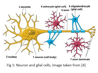
A mechanistic model for neurovascular coupling constitutes a system of differential equations describing the events that occur at a neuronal level during neurovascular coupling. Functional hyperemia is the scientific term describing the stimulus-related increase in blood flow introduced in the previous section. A basic understanding of information processing in the brain is required to interpret the differential equations describing the coupling process. First, there are two types of cells in the brain - neurons and glial cells⁴. Neurons are the cells that send and receive signals while the glial cells support neuronal activities. Everything we think, feel and do would be impossible without the work of neurons and their support cells i.e. the glial cells. Astrocytes are the most numerous kinds of glial cells in the brain.

Action Potential is the fundamental unit of communication between two neurons. A “spike” or an action potential is said to occur when the neuron’s membrane potential reaches $-50mV$. It is a brief electrical event generated in the axon that signals the neuron as ‘active’. This raises the question - why is there a potential difference across the neuron’s membrane? Basic chemistry tells us that when substances are allowed to diffuse freely, they move along the concentration gradient i.e. from regions of high concentration to areas of low concentration until equilibrium is attained. However, neuronal membranes prevent the free distribution of ions along the concentration gradient. Instead, these membranes have proteins called ion channels and pumps that control the movement of ions across the membrane. These ion channels are selective i.e. only some ions can pass through specific channels which open/close in response to specific molecular cues. Due to pumps, which transport ions against their concentration gradient, ions are distributed unequally inside and outside the neuron’s membranes. This unequal charge distribution results in a resting electrical potential difference between the inside and outside of the membrane.

⁵

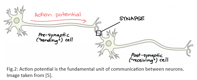
The membrane potential of a neuron is not constant. The instantaneous membrane potential of a neuron depends on all the inputs it receives from the axons of other neurons. An action potential travels the length of the axon and causes the release of chemicals called neurotransmitters into the synapse. The action potential, together with the release of neurotransmitters, enables communication between neurons. Synapse can be thought of as converting an electrical signal (action potential) into a chemical signal (neurotransmitters) and back to the electrical form in the next neuron. Notice in Figure 3 that neurotransmitters are released from the pre-synaptic terminal of one neuron to the post-synaptic terminal of the connected neuron.

⁶

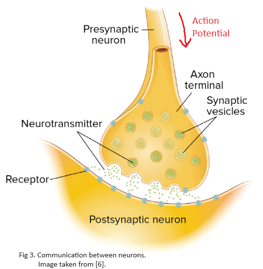
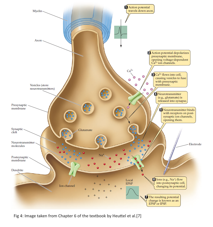
Neurotransmitters are called excitatory neurotransmitters if they make a neuron’s membrane potential more positive (e.g. $-70mV$ to $-60mV$). Glutamate is the most common excitatory neurotransmitter in the brain due to its depolarizing nature. Similarly, inhibitory neurotransmitters make the neuron’s membrane potential more negative. GABA ($\gamma$-aminobutyric acid) is one of the most important inhibitory neurotransmitters that has a hyperpolarizing nature on neurons. Different neurotransmitters attach to different pumps and/or ion channels on the post-synaptic terminal. Figure 4 provides a summary of how neurons “spike” via the release of neurotransmitters. Step-by-step modeling of this biological process is provided.

⁷

1. Action potential travels down the axon i.e. the pre-synaptic terminal experiences a signal as a reduction in membrane potential to $\approx -50mV$. This signal is modeled using the $Stimulus$ function:

   \[Stimulus(t) = k \cdot \mathbb{I}( \text{ } t \in [t_{on}, t_{off}] \text{ }) \quad \quad \quad \cdots Eq \text{ } 1\]
2. Ion channels selective for $Ca^{2+}$ open after experiencing the signal i.e. $Ca^{2+}$ enters the pre-synaptic terminal.
3. There are sac-like structures called vesicles that encapsulate glutamate in the neuron. Entry of $Ca^{2+}$ ions initiates a process that migrates the vesicles to fuse with the pre-synaptic terminal and eventually release glutamate into the synaptic cleft.
4. Glutamate acts as a precursor for GABA. In other words, GABA is formed from glutamate by adding glutamate decarboxylase and vitamin B6⁸. Note that GABA is formed in vivo by a metabolic pathway referred to as the GABA shunt⁹. Entry of $Ca^{2+}$ depolarizes the pre-synaptic neuron and stimulates the release of GABA into the synaptic cleft.

5. Glutamate and GABA diffuse across the synaptic cleft to interact with different receptors on the post-synaptic cleft. Interaction with receptors opens ion channels for the post-synaptic neuron. This can be mathematically modeled under the assumption that GABA and glutamate are the brain’s only inhibitory and excitatory neurotransmitters. \(\frac{\mathrm{d}[Glut]}{\mathrm{d}t} = k_{Glut} \cdot Stimulus(t) - sink_{Glut} \cdot [Glut] \quad \quad \quad \cdots Eq \text{ } 2.1\)

   \[\frac{\mathrm{d}[GABA]}{\mathrm{d}t} = k_{GABA} \cdot Stimulus(t) - sink_{GABA} \cdot [GABA] \quad \quad \quad \cdots Eq \text{ } 2.2\]
6. Glutamate interacts with receptors which activate ion channels that allow an influx of different cations. Therefore, glutamate depolarizes the neuron i.e. makes it more likely for the neuron to fire. On the other hand, GABA interacts with receptors that activate ion channels to hyperpolarize the neuron i.e. they make the neuron less likely to fire. Therefore, the net polarization of a neuron and its probability to fire depends on the net effect of glutamate and GABA coming from connected neurons.

Role of Astrocytes

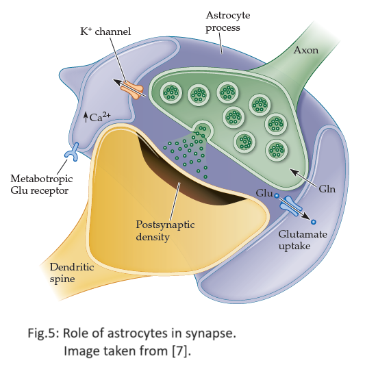
After “sufficient” depolarization of the neuron due to Glutamate’s interaction with its receptor, certain voltage-dependent ion channels for $Ca^{2+}$ open up, allowing for an influx of $Ca^{2+}$ ions into the astrocyte process. In other words, Glutamate increases the concentration of astrocytic $Ca^{2+}$. On the other hand, GABA binds to the $\mathrm{GABA}_{A}$ receptor which reduces the probability of opening the ion channels associated with astrocytic $Ca^{2+}$. Hence, GABA controls the astrocytic $Ca^{2+}$ concentration. The involvement of astrocytes is illustrated in Figure 5.

⁷

Note that the inhibitory actions of GABA become more effective in the presence of a drug called Diazepam. The concentration of astrocytic $Ca^{2+}$, denoted by $[Ca^{2+}]$, in the presence of Diazepam is modeled using the following equation:

\[\frac{\mathrm{d}[Ca^{2+}]}{\mathrm{d}t} = k_{Ca} \cdot (1 + k_3 [Glut]) \left( 1 + \dfrac{[GABA]}{k_4}\left [ 1 + \dfrac{1}{1 + \frac{k^{n}_D}{c^{n}_D} } \right] \right) - sink_{Ca}[Ca^{2+}] \quad \quad \cdots Eq \text{ } 3\]

In the equation describing astrocytic $Ca^{2+}$ concentration,

• $k_3, k_4, sink_{Ca}$ and $kk_{Ca}$ are kinetic rate parameters measured in $mol ml^{-1} sec^{-1}$.
• $c_D$ denotes the blood plasma concentration of diazepam.
• $k_D$ denotes the dissociation coefficient while $n$ is the Hill coefficient.

Notice that Equation 3 models GABA and glutamate’s inhibitory and excitatory relationship with astrocytic $Ca^{2+}$ based on whether the terms $[GABA]$ and $[Glut]$ are in the numerator or denominator. Additionally, the term \dfrac{1}{1 + \frac{k^{n}_D}{c^{n}_D}, multiplied to $[GABA]$, models the boosted inhibitory nature of $GABA$ in the presence of diazepam.

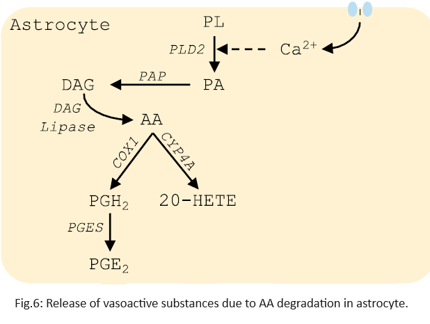
An increase in astrocytic $Ca^{2+}$ concentration initiates an enzymatic process, eventually increasing intracellular Arachidonic Acid (AA). Figure 6 gives a slightly more detailed picture of AA formation. For mathematical simplicity, these details are ignored and AA concentration is modeled as follows:

\[\frac{\mathrm{d}[AA]}{\mathrm{d}t} = k_{pl}[Ca^{2+}] - (k_{vc} + k_{vd})[AA] \quad \quad \quad \cdots Eq \text{ } 4$\]

• The rate constant $k_{pl}$ models the crease in $[AA]$ with an increase in $[Ca^{2+}]$.
• The constants $k_{vc}$ and $k_{vd}$ model the degradation or transformation of AA into different vasoactive substances i.e. the substances that increase/decrease the blood vessel’s diameter. Vasoactive substances can promote vasodilation (increase diameter, Eg. $PGE_2$) or vasoconstriction (reduce the diameter, Eg. $20-HETE$).

The release of these vasoactive substances controls blood flow and blood volume, which starts the vascular side of hemodynamics. This blood flow in turn controls the amount of oxyhemoglobin ($oHb$), deoxyhemoglobin (dHb), oxygen ($O_2$), and glucose flowing in and out of the local blood vessel³.

³

It has been established previously that blood flow ($v_{flow}$) and blood volume ($v_{bv}$) have a non-linear relationship³. The authors model this non-linear relationship as follows:

\[v_{bv} = (v_{flow})^{k_bv}\]