SECT statistic

Introduction to Persistence Diagrams

The objective of this blog post is to summarize my understanding of the theory and applications behind Smooth Euler Characteristic Transform (SECT) statistic which was first introduced by Crawford et al¹ in 2020. The SECT statistic summarizes the shape information associated with an object as a collection of smooth curves that lie in a Hilbert space. The “niceness” of a Hilbert space allows us to use different tools from Functional Data Analysis (FDA). The motivation behind SECT comes from the Persistent Homology Transform (PHT) statistic introduced by Turner et al² in 2014. The blog post starts with a review of Persistence Diagram basics, followed by an introduction to PHT, its properties, and drawbacks. The third section discusses the benefits of having a Hilbert space structure from a statistics point of view. The fourth and final section discusses the construction of SECT statistic.

Assume that we are given a finite simplicial complex $\mathcal{K}$ along with its corresponding filteration $\mathcal{F} = \lbrace K_1, K_2, \cdots \rbrace$. A simplicial $k$-chain is a $\mathbb{F}$-linear combination of $k$-simplices in $\mathcal{K}$ for some choice of field $\mathcal{F}$. The set of all such $k$-chains form the vector space $C_k(\mathcal{K})$. This vector space is required to define the $k$-th boundary map $\partial_k$ of $\mathcal{K}$.

\[\partial_k : C_k(\mathcal{K}) \longrightarrow C_{k-1}(\mathcal{K}) \quad \text{ where } \quad \[v_0, v_1, \cdots, v_k \] \longmapsto \sum_{j=0}^k (-1)^j \[ v_0, v_1, \cdots, v_{j-1}, v_{j}, \cdots v_k \]\]

The $k$-th Homology group is then defined as:

\[H_k(\mathcal{K}) = \dfrac{\text{Ker}(\partial_k)}{\text{Im}(\partial_{k+1})}\]

Persistence diagrams summarize how the topology of $\mathcal{K}$ changes with respect to the filteration $\mathcal{F}$. For the homology class $\alpha \in H_k(K_i)$,the quantity $\mathrm{d}(\alpha) - \mathrm{b}(\alpha)$ defines persistence of class $\alpha$ where $\mathrm{d}(\alpha)$ and $\mathrm{b}(\alpha)$ denote the “birth” and “death” time (or the filteration number) of the equivalence class $\alpha$.

Persistent Homology Transform (PHT)

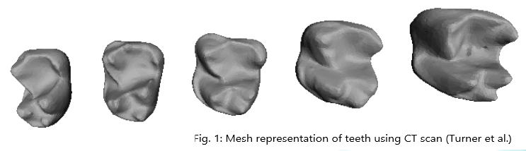
The authors of both PHT² and SECT¹ are trying to tackle the problem of how shape information can be quantified in a way that enables us to perform statistical inference. The PHT statistic, introduced by Turner et al², is to model objects in $\mathbb{R}^2$ and $\mathbb{R}^3$. PHT captures shape information as a collection of Persistent Diagrams that we have to work with instead of the object itself. Hence, the resulting space of persistence diagrams, $\mathcal{D}$, needs to be “nice” i.e. a space where we can perform statistical inference. For instance, consider the CT scan mesh representations of five teeth taken from Turner et al². If there exists a distance function $d$ such that $(\mathcal{D}, d)$ is a well-defined metric space, then such a metric $d$ could be used to compare the shapes of these teeth.

A detailed introduction to Persistence Diagrams can be found in the third chapter of the textbook by Dey and Wang ³. Let $M \subset \mathbb{R}^d$ be such that it can be approximated using a finite simplicial complex. The set of all possible (unit vector) directions in $\mathbb{R}^d$ lie in the $d-1$ sphere $\mathcal{S}^{d-1} \subset \mathbb{R}^d$. Additionally, for a fixed $v \in \mathcal{S}^{d-1}$, $M(v)$ will denote the projection of points in M onto the vector $v$.

\[\mathcal{S}^{d-1} = \lbrace x \in \mathbb{R}^d \text{ } : \text{ } \|\| x \|\|_{2} = 1 \rbrace \quad \text{ and } \quad M(v) \triangleq \lbrace x \cdot v \text{ } : \text{ } x \in M \rbrace \text{ for fixed } v \in \mathcal{S}^{d-1}\]

For each such $v$, we can define a filtration $\lbrace M(v)_{r} : r>0 \rbrace$ (w.r.t. the height function) indexed by height $r$ such that $M(v)_r$ corresponds to the subset of $M$ that is atmost at height $r$, from the baseline, in the direction of $v$.

\[M(v)_r = \lbrace x \in M : x \cdot v \leq r \rbrace \text{ for } r \geq 0\]

For a fixed $v$, topological information in the direction of this vector can be summarized using persistence diagrams associated with the filtration $\lbrace M(v)_{r}: r>0 \rbrace$ (w.r.t height). Intuitively the corresponding persistence diagrams, denoted by $X_k(M,v)$ for $k \in \lbrace 0, 1, \cdots , d-1 \rbrace $, store topological information ( w.r.t. height ) along the direction $v$. Therefore collecting the persistence diagrams $X_k(M,v)$ for all $k$ and all directions $v \in \mathcal{S}^{d-1}$ will contain all possible topological information. This is the intuition behind the Persistent Homology transform of $M$, denoted as $PHT(M)$:

\[PHT(M): \mathcal{S}^{d-1} \longrightarrow \mathcal{D}^d\] \[\quad \quad \quad \quad \quad\quad \quad \quad \quad \quad \quad \quad \quad \quad \quad \quad \quad \quad \quad \quad v \longmapsto (X_0(M,v), X_1(M,v), \cdots, X_{d-1}(M,v))\]

Note that $PHT(M)$ cannot be all possible topological information associated with $M$, instead, the information we have access to is restricted by the choice of filter function (here, it is the height function) and filtration.

Construction of SECT statistic