Introduction to Mixtures Models
Data is often a heterogeneous mix of different types of groups. In such scenarios, we need variable(s) to identify the group or category to which the data point belongs. Finite mixture models are a popular choice to model data with known/unknown group structures. If the group structure is known, we have a classification problem while an unknown group structure points to a clustering problem. Generally, finite mixtures model data to be coming from a known/unknown number of parametric densities. This modeling assumption makes finite mixture models an intuitive choice for density estimation as well. For instance, skewed or heavy-tailed histograms might be better approximated using finite mixtures than symmetric distributions like the normal distribution.
Karl Pearson, in 1894, was among the first to employ finite mixture models to analyze crab data provided by the evolutionary biologist Weldon. The crab data consisted of measurements of the forehead to body length of a thousand crabs sampled from the Bay of Naples. Each of these measurements falls into one of 29 interval categories. This dataset is saved as the dataframe pearson in the R Package mixdist. Look at the link1 to learn more about the data analysis. Pearson assumed that forehead-to-body length ratios are sampled from a mixture of two normal densities with different means and variances. Pearson used the method of moments to estimate the mean and variance parameters. This involved solving a ninth-degree polynomial by hand. Clearly, due to a lack of computational power, finite mixture models weren’t studied as much until the advent of computers. The advent of computers and a better understanding of the properties of the maximum likelihood function in the case of normal components led to an eventual increase in the use of mixture models. However, it was the paper introducing the EM algorithm (1977) that greatly stimulated interest in using finite mixtures to model heterogeneous data.2
Mixture Model formulation
If we model the data $\mathbf{Y} \in \mathbb{R}^n$ is drawn from a mixture distribution containing $G$ parametric component densities $f(\cdot ; \theta_i)$ with proportions $\pi_i$, then
\[\mathbf{Y} \sim \sum_{i=1}^G \pi_i f(\mathbf{y}; \theta_i) \quad \text{ where } \quad \sum_{j=1}^G \pi_j = 1 \quad \theta_i \in \Theta \forall \text{ } i \in \lbrace 1, \cdots, G \rbrace \text{ and } G \in \mathbb{N} \cup \lbrace \infty \rbrace \quad \quad ---(1)\]Notice that in definition (1), we let $G \in \mathbb{N} \cup \lbrace \infty \rbrace$ i.e. we can use a finite or countably infinite number of components in the mixture model. Equivalently, mixture models can be interpreted as the expectation with respect to a mixing measure $H$. Here, one can define $H$ to be a measure with finite or countable support that places weight $\pi_j$ at position $\theta_j$. A point mass at $\theta \in \Theta$ is denoted using the indicator function $\mathbb{1}_{\theta}$. Note that (1) and (2) are equivalent representations of a mixture model.
\[\mathbf{Y} \sim \int_{\Theta} f(\text{ }\cdot \text{ } ; \theta ) H(\mathrm{d}\theta) \quad \text{ where } \quad H = \sum_{i=1}^G \pi_i \mathbb{1}_{\theta_i} \quad \quad ---(2)\]Notice that models (1) and (2) assume that all components belong to the same family of a parametric distribution. This is a commonly used assumption for mixture models. However, one can generalize model (1) by letting the $i$-th component come from density $f_i$ with parameter $\theta_i$. This gives a generalization of the model (1) which no longer has the expectation interpretation.3
There are two common interpretations of mixture models with at most countably many components. According to Chapter 1 of “Handbook of Mixture Analysis”, one of the interpretations is more probabilistic while the other is more analytic. In either case, the model stays the same:
\[Y_i | Z_i = z_i \sim f(\text{ } \cdot \text{ }| \theta_{z_i} ) \quad \text{ where } \quad Z_i \sim \sum_{j=1}^G \pi_j \mathbb{1}_{j} \quad \quad ---(3)\]- Probabilistic interpretation: We assume that the population is truly heterogeneous and the $G$ components correspond to $G$ distinct sub-populations of interest that are present in populations $(\pi_1, \pi_2, \cdots, \pi_G)^T$. A random draw from the distribution is a draw from the $i$-th component with probability $\pi_i$. Depending on whether $G$ is known or unknown, we have a classification or clustering problem.
- Analytic interpretation: The latent variable representation might be a convenient modeling choice even though there is no “real” sub-group structure within the data.
Model (3) involves the latent variable (or allocation variable) $Z_i$ since it is unobserved. Now, given a mixture model of the type (3), there are two common ways of inferring unknown parameters $G$ (if it is unknown), $\mathbf{\theta} = (\theta_1, \cdots, \theta_G)^T,$ and $\mathbf{\pi} = (\pi_1, \cdots, \pi_G)$ - Frequentist approach vs Bayesian approach.
| Frequentist | Bayesian parametric | Bayesian non-parametric |
|---|---|---|
| $\mathbf{Y} \sim \sum_{i=1}^G \pi_i f(\mathbf{y}; \theta_{z_i})$ where $\mathbf{\theta}, \mathbf{\pi}$ and $G$ are assumed fixed but unknown |
$\mathbf{Y} \mid Z_i = z_i \sim f(\mathbf{y}; \theta_i)$ $Z_i \mid \mathbf{\pi} \sim Multinom(\mathbf{\pi})$ $\mathbf{\pi} \sim Dir(\alpha_0)$ for known $\alpha_0$ |
$\mathbf{Y} \mid H \sim \int_{\Theta} f(\text{ }\cdot \text{ } ; \theta ) H(\mathrm{d}\theta)$ $H \sim \mathcal{F}$ where $\mathcal{F}$ is a well-defined distribution over probability measures. |
| Mixing measure $H$ is deterministic and unknown | Mixing measure $H$ is a known parametric density with random parameters | Mixing measure $H$ is an unknown non-parametric density. |
| EM algorithm is used to perform maximum likelihood estimation | Use MCMC methods for posterior inference | Use MCMC methods for posterior inference |
Dirichlet Processes
Dirichlet Process Mixture Model is a Bayesian non-parametric technique that requires a probability distribution defined over a set of probability measures, say $\mathcal{F}$. Dirichlet Processes (DP) is a popular choice for $\mathcal{F}$ in Bayesian non-parametric settings. Note that a random draw from a DP is a probability measure that cannot be described using a finite number of parameters. Moreover, DP priors ensure tractable posterior computations as well.4
Let $G$ be a random measure over $\Theta$ i.e. $G: \Theta \longrightarrow [0,1]$. Then for $\alpha >0$ and a distribution $H:\Theta \longrightarrow [0,1]$, we say that $G \sim DP(\alpha, H)$ if for any measurable partition $\lbrace A_1, \cdots,A_r \rbrace$ of $\Theta$ we have:
\[(G(A_1), G(A_2), \cdots, G(A_r)) \sim Dir(\alpha H(A), \alpha H(A_2), \cdots, \alpha H(A_r))\]Notice that $H(A)$ is again a random variable for any measurable set $A \subseteq \Theta$. Moreover, the following two properties will provide an intuitive interpretation for $\alpha$ and $H$.
- $\mathbb{E}[G(A)] = H(A)$ for measurable set $A \subseteq \Theta$.
- $Var[G(A)] = \dfrac{H(A)[1-H(A)]}{\alpha + 1}$
Fig 1: Samples from $DP(\alpha, H)$ for four different $\alpha$ values and $H \equiv Pois(4)$. Python code used to generate the plot is based on PyMC documentation.5
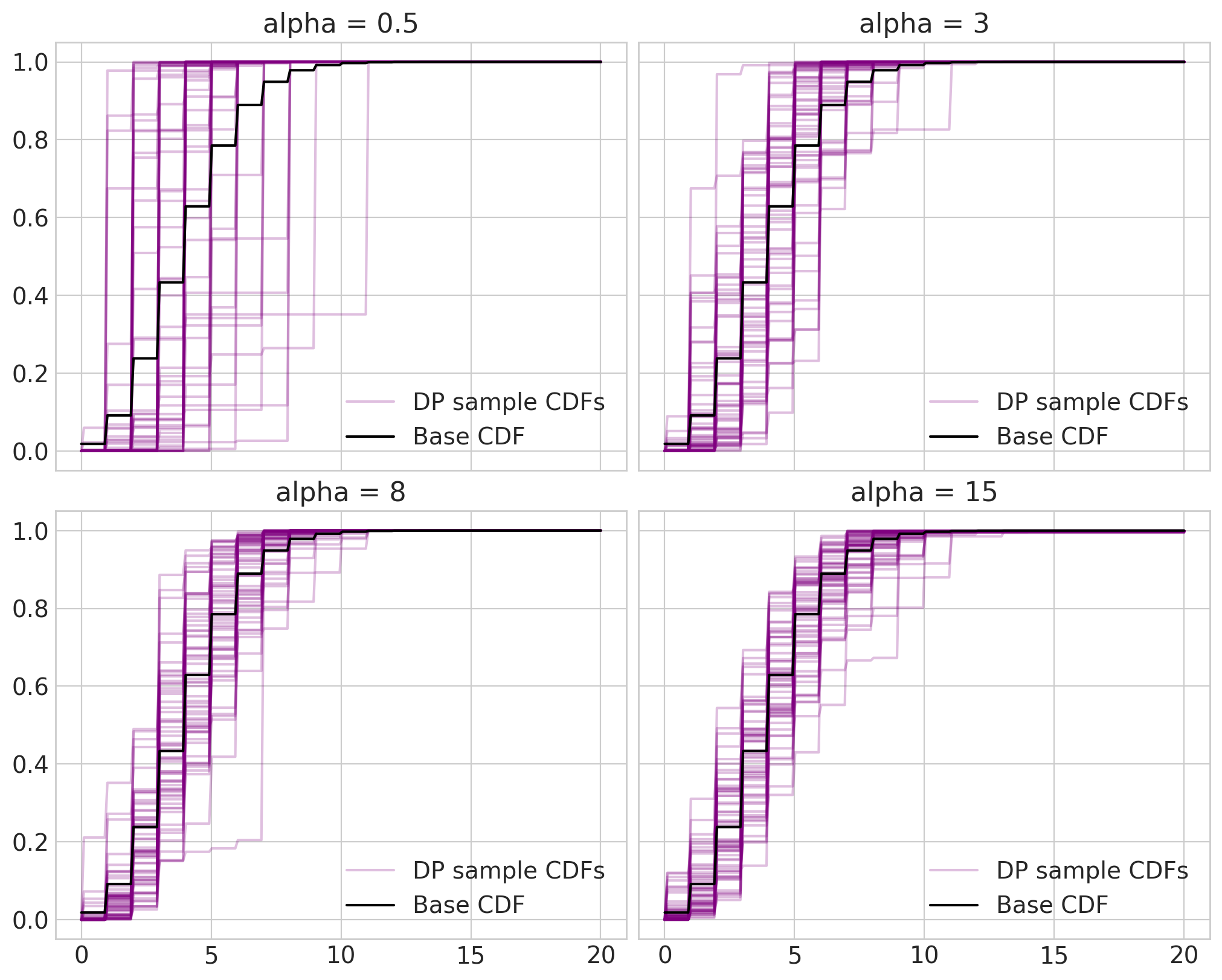
From Figure 1, it is clear that the base measure $H$ plays the role of average i.e. draws from the DP are centered around $H$. On the other hand, $\alpha$ quantifies inverse variance. In case of a larger $\alpha$, a draw from the DP will have its mass concentrated closer to and around $H$. For this reason, $\alpha$ is called concentration parameter or strength parameter. Figure 1 also shows that DP samples “converge” (not mathematically rigorous) to the base distribution $H$ as $\alpha \longrightarrow \infty$.
Posterior and Predictive distributions
Let $G \sim DP(\alpha)$ where $G: \Theta \longrightarrow [0,1]$ is a random measure
Let $\theta_1, \theta_2, \cdots, \theta_n \overset{\mathrm{iid}}{\sim} G$
- The posterior distribution is a weighted sum of prior and empirical distributions.
- We know that $\theta_{n+1} \Big \vert G, \theta_1, \cdots, \theta_n \sim G$. Then,
Beta distribution, Dirichlet distribution, and Dirichlet Process
A random draw $\rho$ from $Beta(a,b)$ corresponds to a distribution over two categories. For instance, if $\rho = 0.7$, then the corresponding distribution places a weight $0.7$ on category 1 and weight $0.3$ on category 2. The parameters $a$ and $b$ quantify the measure of weights placed at categories 1 and 2 respectively. Depending on parameter values $a$ and $b$, beta density can be symmetric or asymmetric and bounded or unbounded. Note that $Beta(1,1)$ is equivalent to $Unif(0,1)$.
Fig 2: Beta density plots for different values of parameters: $\alpha$ and $\beta$.

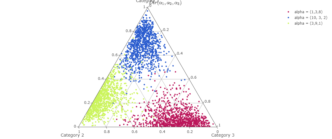
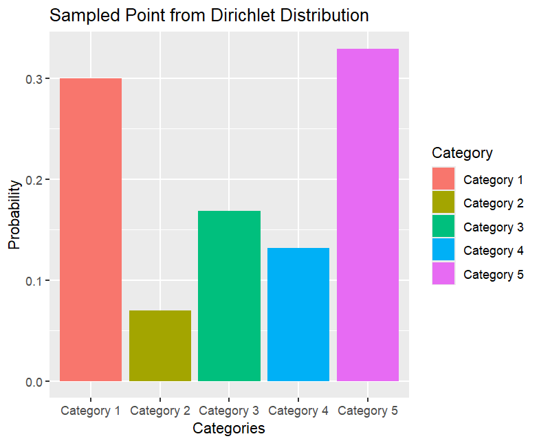
Dirichlet Distribution is a generalization of Beta distribution to $K$ categories. Just like the Beta distribution is defined on the $1$-simplex, the Dirichlet distribution is defined on a $(K-1)$-simplex. If $\rho$ is sampled from a Dirichlet distribution with $K$-dimensional parameter $\alpha$, then the realization $\rho = (\rho_1, \cdots, \rho_K)^T$ is such that its components add up to 1. Just like a draw from the Beta distribution corresponds to a discrete distribution on two categories, a draw from $Dir(\alpha)$ with $\alpha \in \mathbb{R}^K$ corresponds to a discrete distribution over $K$ categories. The constituents of parameter $\alpha = (\alpha_1, \alpha_2, \cdots, \alpha_K)^T$ quantify the measure of weights at each of the $K$ categories.
Fig 3: Samples from Dirichlet distribution for different concentration parameter values. Plots have been made using Plotly’s documentation on ternery plots6.

To begin with, there is a difference between the number of “clusters” and the number of “components”. A given component of the finite mixture model is a cluster if at least one data point is assigned to the component. Hence, if we are working with a $4$-component mixture model, there are $4$ possible components in total. Moreover, given a data set, $4$ clusters can be formed at most. This might tempt one to think that choosing a large but finite $K$ is appropriate. However, this is incorrect since, given a fixed $K$, we will eventually fill all components if we have a “large enough” sample size.7 This issue is resolved in a DPMM by setting $K \longrightarrow \infty$. Although it seems counterintuitive at the moment, this should make sense by the end of the blog post. Setting $K \longrightarrow \infty$ leads to a new problem - how do we construct a sequence of proportions $\lbrace \rho_i \rbrace_{i \in \mathbb{N}}$ such that $\sum_{i \in \mathbb{N}} \rho_i = 1$.
| Distribution | A random sample from the distribution | Comments |
|---|---|---|
| $\rho_1 \sim Beta(\alpha_1, \alpha_2)$ $\rho_2 = 1 - \rho_1$ $\alpha_1, \alpha_2 >0$ |
 |
A random draw $\rho \sim Beta(\alpha_1, \alpha_2)$ corresponds to the pmf $(\rho, 1 - \rho)$ |
| $\vec{\mathbf{\rho}} \sim Dir(\alpha_1, \alpha_2, \cdots, \alpha_K)$ where $\alpha_i >0 \forall i = 1, \cdots, N$. Then, $\vec{\rho}$ is $K$-dimensional and $\sum_{i=1}^K \rho_i = 1$ |
 |
A random draw $\vec{\rho} \sim Dir(\alpha_1, \cdots, \alpha_K)$ corresponds to the pmf $(\rho_1, \rho_2, \cdots, \rho_K)$ |
| $\vec{\mathbf{\rho}} \sim GEM(\alpha)$ for $\alpha >0$ Then $\vec{\rho}$ corresponds to the sequence $\lbrace \rho_i \rbrace_{i \in \mathbb{N}}$ which satisfies $\sum_{i \in \mathbb{N}} \rho_i = 1$ |
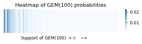 |
A random draw $\vec{\rho} \sim GEM(\alpha)$ corresponds to the pmf $\lbrace \rho_i : i \in \mathbb{N} \rbrace$ such that $\sum_{i} \in \mathbb{N} \rho_i = 1$ |
| $G \sim DP(\alpha, G_0)$ for $\alpha >0 $and base measure $G_0: \Theta \longrightarrow [0,1]$. Then $G = \sum_{i \in \mathbb{N}} \rho_i \mathbb{1}_{\phi_i}$ w.p. $1$ for some $\vec{\mathbf{\rho}} \sim GEM(\alpha)$ and $\phi_1, \phi_2, \cdots \overset{\mathrm{iid}}{\sim} G_0$ |
aaa | aaa |
GEM to DPMM
Chinese Restaurant Process
about CRP and the Blackwell-Mac Queen scheme.
Moreover, finite mixture models have theoretical guarantees to justify their usefulness. One of the most recently proven theoretical guarantees I found is by Nguyen et al8. The main theorem Nguyen et al proved is given below. Refer to Theorem 2.1 in the article8 for rigorous mathematical details.
Theorem
Let $f$ and $g$ be continuous probability densities on $\mathbb{R}^n$ i.e. $f,g: \mathbb{R}^n \longrightarrow \mathbb{R}$. Define the set of $m$-component location-scale finite mixture of the PDF $g$ as follows:
\[\mathcal{M}^g_m = \left \lbrace h^g_m \quad : \quad h^g_m(x) := \sum_{i=1}^m c_i \frac{1}{\sigma_i^n} g\left(\frac{x - \mu_i}{\sigma_i}\right) \text{ such that } \mu_i \in \mathbb{R}^n, \sigma_i > 0 \forall i \text{ and } \sum_{j=1}^m c_i = 1 \right \rbrace\]Further, let $\mathcal{M}^g := \bigcup_{m \in \mathbb{N}} \mathcal{M}^g_m$. Then the following statements are true:
- Let $\mathbb{K} \subset \mathbb{R}^n$ be a compact set. Then there exists a sequence of functions $\left \lbrace h_{m}^g \right \rbrace_{m \in \mathbb{N}}$ such that $h_{m}^g \in \mathcal{M}^g$ for each $g \in \mathbb{N}$ and
- For $p>1$, if $f \in \mathcal{L_p} \text{ and } g \in \mathcal{L_{\infty}}$, then there exists a sequence of functions $\left \lbrace h_{m}^g \right \rbrace_{m \in \mathbb{N}}$ such that $h_{m}^g \in \mathcal{M}^g$ for each $g \in \mathbb{N}$ and
Therefore, a mixture model can arbitrarily approximate complex densities by choosing the right component distributions. This theorem (and similar results proven earlier) can be seen as the motivation behind why it makes sense to look at mixture models with $G \longrightarrow \infty$. Setting the number of components to infinity solves another problem associated with mixture models. Let us say that we are working with a $G$-component finite mixture model. Then, if we have data that is “large enough”, the finite mixture model will eventually fit all data into the $G$ components.
Some Mixture Model variations
So far, we looked at mixture models with at most countably many components. However, this definition can be generalized further by allowing the mixing measure to be discrete or continuous. So far, we let $H$ represent a discrete probability measure. Assume for instance that $H$ represents Beta CDF with parameters $\theta = (\alpha, \beta)^T$
\[Y | H = h \sim Binom(N, h) \quad \text{ and } \quad H \sim Beta(\alpha, \beta) \quad \implies \quad f(h|Y=y) \propto \int_{p \in [0,1]} h^y (1-h)^{N-y} H(\mathrm{d}h)\]This is an example of a continuous mixture where we “mix” the binomial density w.r.t. beta distribution. Notice that this is nothing but Beta-Binomial conjugacy. Like the Beta-Binomial example, the conjugacy examples we often see in introductory Bayesian statistics are all examples of continuous mixtures. Most examples we see are exponential family models “mixed” by their conjugate priors.3 Some mixture model generalizations or variations not discussed here are mixture of experts models, finite mixtures with non-parametric components, hidden Markov models, and spatial mixtures. Refer to “Handbook of Mixture Analysis”3 to learn about these mixture model variations.
Bayesian non-parametric mixtures
Points to include
- Bayesian vs frequentist mixtures (H random vs deterministic with unknown params)
- Dirichlet distribution also has two interpretations (just like mixture models)
- Dirichlet distribution to Dirichlet process
- Components vs clusters
- At what rate do clusters grow wrt sample size?
- Bayesian mixture model inference is of two types - within and across model sampling. Reversible jump MCMC is an example of across model sampling.
- Mention primary reference 7
References
-
Karl Pearson and the crabs from Naples bay, Francesco Pasqualini ↩
-
McLachlan, G., and Peel, D. (2000), “Finite Mixture Models,” Wiley Series in Probability and Statistics, Wiley. DOI: 10.1002/0471721182 ↩
-
Frühwirth-Schnatter, S., Celeux, G., and Robert, C. P. (eds.) (2019), Handbook of Mixture Analysis, Chapman and Hall/CRC. DOI: https://doi.org/10.1201/9780429055911. ↩ ↩2 ↩3
-
Teh, Y. (2011). Dirichlet Process. In: Sammut, C., Webb, G.I. (eds) Encyclopedia of Machine Learning. Springer, Boston, MA. DOI: https://doi.org/10.1007/978-0-387-30164-8_219. Also available as lecture notes on Yee Whye Teh’s website ↩
-
Dirichlet process mixtures for density estimation, PyMC documentation. Last seen: 17th Sept, 2024. ↩
-
Making ternary plots using the
Plotlypackage: https://plotly.com/r/ternary-plots/ ↩ -
Nonparametric Bayes Tutorial offered by Tamara Broderick, Machine Learning Summer School (MLSS), 2006 ↩ ↩2
-
Nguyen, T., Chamroukhi, F., Nguyen, H. D., and McLachlan, G. J. (2022), “Approximation of probability density functions via location-scale finite mixtures in Lebesgue spaces,” Communications in Statistics - Theory and Methods, Informa UK Limited. DOI: 10.1080/03610926.2021.2002360. ↩ ↩2